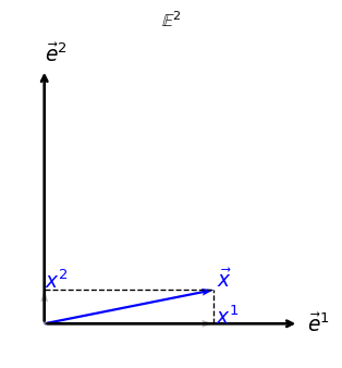
Each component \(x^i\) corresponds to the projection of \(\vec{x}\) onto the corresponding basis vector \(\vec{e}^i\). These components carry physical meaning: they represent distances measured along fixed spatial directions from the origin.
To simplify visualization, we consider a 2-dimensional slice, \(\mathbb{E}^2\), where:
\[
\vec{x} = (x^1, x^2)
\]
Below, we illustrate a vector \(\vec{x}\) in \(\mathbb{E}^2\), decomposed into its components.
Figure 1: In this diagram, \(\vec{x}\) is shown along with its projections onto the \(x^1\) and \(x^2\) axes. The dashed lines and gray arrows indicate the coordinate decomposition that defines the Cartesian components.
Time
So far, we’ve discussed a single static space, like a snapshot of the world frozen at a particular instant. In such a snapshot, distances and directions are described by a Euclidean space, \(\mathbb{E}^2\) or \(\mathbb{E}^3\).
But time enters physics through measurement: We don’t just measure where things are, we also measure when.
Two Roles of Time
Time appears in two distinct but related ways:
Simultaneity: We want to compare the positions of multiple objects at the same instant. For example: “Two cars are 10 meters apart at 12:00.”
Change: We want to track how the position of something evolves over time. For example: “This car was at \(\vec{x}_0\) at 12:00 and at \(\vec{x}_1\) at 12:05.”
This second case introduces a subtle question:
What Does It Mean for a Point to Stay in the Same Place?
To say something “moved” from \(\vec{x}_0\) to \(\vec{x}_1\), we must assume:
“The point that was at \(\vec{x}_0\) at time \(t_0\) is the same place as the one at \(\vec{x}_1\) at time \(t_1\).”
But how do we decide that?
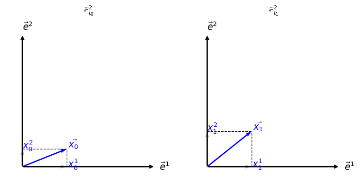
Each snapshot in time is a separate space, like \(\mathbb{E}^2_{t_0}\) and \(\mathbb{E}^2_{t_1}\). To describe motion, we must define a rule that identifies points across these spaces.
Each figure is a full space at a fixed time: a spatial snapshot. But motion requires more than snapshots: it requires a way to track points across time.
The Identity Map (Trivial Frame)
To describe motion, we need to track spatial points across time: we must decide what it means for a point at time \(t_0\) to be “the same place” as a point at time \(t_1\).
Let’s consider a simple scenario:
An observer is in a room and chooses a particular corner to serve as the origin of their coordinate system. From this origin, they align three fixed axes, say, along the edges of the room, and assign coordinates to every point based on measured distances along these axes.
Now suppose this same observer makes two measurements, at times \(t_0\) and \(t_1\), using the same reference system: the same corner, the same directions, and the same notion of distance. Then, the observer naturally identifies the “same point in space” at both times by matching coordinates: \[
\vec{x}_1 = \vec{x}_0
\]
This defines the so-called identity map (or trivial identification): \[
\phi: \mathbb{E}^2_{t_0} \to \mathbb{E}^2_{t_1}, \qquad \phi(\vec{x}_0) = \vec{x}_0
\]
Under this rule, an object is said to remain at rest if its coordinates do not change with time. However, this identification is not absolute, it is tied to the specific reference system used by the observer.
This distinction is key:
The first part of our discussion (assigning coordinates) requires physical references: like walls, corners, rulers; to define positions at a single instant.
The second part (relating points across time) defines the reference frame: the rule we use to track positions through time.
In practice, when we draw diagrams in \(\mathbb{E}^2\), we often implicitly assume this trivial map, we imagine the reference objects do not move over time. This allows us to focus on how other objects evolve relative to the fixed background.
But this is only one possibility. More general mappings reflect different frames of reference, for example, frames moving with constant velocity (Galilean boosts). We’ll return to this idea soon.
Maps Must Reflect Physical Expectations
Once we allow more general observers or motion, we must impose some physical conditions on the maps we use between spatial snapshots.
These come from our experience with the physical world, and how we expect objects to move and interact:
Points must not collide: If two distinct points at time \(t_0\) map to the same point at \(t_1\), we cannot distinguish their identities anymore. This contradicts the idea that particles have individual, continuous paths.
No points should appear or vanish: Every point at \(t_1\) must correspond to a point at \(t_0\). Otherwise, matter could appear from nothing or disappear entirely.
From these we conclude:
The map \(\phi: \mathbb{E}^2_{t_0} \to \mathbb{E}^2_{t_1}\) must be bijective (one-to-one and onto).
Furthermore, based on how real objects move, without teleportation or discontinuous jumps, we also expect:
The map should be smooth: small changes in position at \(t_0\) lead to small changes at \(t_1\).
This leads us to model \(\phi\) as a diffeomorphism, a smooth, invertible map with a smooth inverse.
But again: This isn’t a mathematical requirement: it’s a physical modeling assumption based on the continuity of motion observed in nature.
Describing Motion: The Law of Dynamics
Before we can speak of forces or equations of motion, we must clarify what it means for an object to move, and how we can measure that change.
In practice, what we have is a sequence of observations: the position of a particle at different instants of time. Each of these measurements belongs to a copy of space, say \(\mathbb{E}^3_t\), at time \(t\). But to compare them, to say how much the object moved, or how fast it changed direction, we must first decide how to identify points across time.
This is not automatic. It involves a modeling choice, which we made earlier by introducing a map between spatial snapshots. This map tells us which points at different times are considered “the same” from the observer’s perspective. Only then does the notion of displacement make sense.
Once we can compare positions across time, we can take differences, and eventually define the acceleration: \[
\ddot{\vec{x}}(t) = \lim_{\delta t \to 0} \frac{\vec{x}(t + \delta t) + \vec{x}(t - \delta t) - 2\vec{x}(t)}{\delta t^2},
\] where the dot indicates derivatives with respect to time.
Only after setting up this structure, coordinates, maps, and vector space operations, does it become meaningful to introduce Newton’s second law: \[
\vec{F} = m \ddot{\vec{x}}
\] This equation is not the starting point, but rather the culmination of a chain of ideas rooted in observation: we measure position, define displacement and acceleration, and from there, assign a force. Historically, this came from empirical regularities, but here we are unpacking what it means to write such an equation and what assumptions it relies on.
Ultimately, Newton’s law reflects not just an observed pattern, but a whole framework of measurement, a way of tracking objects through space and time using a coherent mathematical model.
Consistency of Vector Operations
To define acceleration, we use the second derivative: \[
\ddot{\vec{x}}(t) = \lim_{\delta t \to 0} \frac{ \vec{x}(t+\delta t) + \vec{x}(t-\delta t) - 2\vec{x}(t) }{\delta t^2}
\] At first glance, this seems like a purely mathematical operation. But for this expression to make sense, we must be able to add and subtract vectors that come from different spaces: \(\vec{x}(t+\delta t) \in \mathbb{E}^3_{t+\delta t}\), \(\vec{x}(t-\delta t) \in \mathbb{E}^3_{t-\delta t}\), and \(\vec{x}(t) \in \mathbb{E}^3_t\).
To do this, we need a rule that tells us how to bring all these vectors into the same vector space so that arithmetic operations are well-defined. This is precisely what our map \(\phi\) does, it tells us how to identify points and vectors between spaces at different times.
When we adopt the trivial map (identity), we are assuming that: \[
\vec{x}(t+\delta t) \in \mathbb{E}^3_{t+\delta t} \quad \text{is mapped to} \quad \mathbb{E}^3_t \quad \text{via} \quad \phi^{-1},
\] and likewise for \(\vec{x}(t-\delta t)\). With this identification, all three vectors are interpreted as elements of \(\mathbb{E}^3_t\), and the derivative is now well defined.
This idea, that to differentiate vectors we must decide how to compare them at different points, is not just a technicality. It is the seed of a deep mathematical concept known as parallel transport, a central idea in differential geometry. There, we study more general rules for transporting vectors across curved spaces, where no global trivial identification exists.
In our case, we are working in flat Euclidean space with a chosen frame, so the identity map suffices. But it’s important to recognize that even here, the notion of transporting vectors is already present, though implicitly. And it is this structure that allows us to go from a sequence of positions to the definition of motion and dynamics.
What if We Could Not Adopt the Identity Map?
So far, we have implicitly assumed that vectors at different times can be directly compared using the identity map. But what if this were not the case? What if comparing vectors at different times required a more general rule?
Let’s define a map \(T_{t_1, t_2}\) that takes a vector from the space at time \(t_1\), denoted \(\mathbb{E}^3_{t_1}\), to the space at time \(t_2\), \(\mathbb{E}^3_{t_2}\). A simple example of such a map is: \[
T_{t_1, t_2} \vec{x} = \vec{x} + \vec{v}(t_2) - \vec{v}(t_1),
\] where \(\vec{v}(t)\) is some vector-valued function of time. This is actually a special case of a more general concept called a diffeomorphism, but this simple form is enough for our discussion.
Now, let’s see how this affects how we define the second derivative. We can write: \[
\frac{\dD^2 \vec{x}}{\dD t^2} = \lim_{\delta t \to 0} \frac{T_{t+\delta t, t} \vec{x}(t + \delta t) + T_{t-\delta t, t} \vec{x}(t - \delta t) - 2 \vec{x}(t)}{\delta t^2}.
\]
To evaluate this, we expand both transported terms using a Taylor series. For small \(\delta t\), we get: \[
\begin{aligned}
T_{t+\delta t, t} \vec{x}(t + \delta t) &= \vec{x}(t + \delta t) + \vec{v}(t) - \vec{v}(t + \delta t) \\
&= \vec{x}(t + \delta t) - \dot{\vec{v}}(t)\delta t - \tfrac{1}{2} \ddot{\vec{v}}(t)\delta t^2 + O(\delta t^3), \\
T_{t-\delta t, t} \vec{x}(t - \delta t) &= \vec{x}(t - \delta t) + \vec{v}(t) - \vec{v}(t - \delta t) \\
&= \vec{x}(t - \delta t) + \dot{\vec{v}}(t)\delta t - \tfrac{1}{2} \ddot{\vec{v}}(t)\delta t^2 + O(\delta t^3).
\end{aligned}
\]
Now plugging these into the expression for the second derivative: \[
\frac{\dD^2 \vec{x}}{\dD t^2} = \lim_{\delta t \to 0} \frac{\vec{x}(t + \delta t) + \vec{x}(t - \delta t) - 2\vec{x}(t) - \ddot{\vec{v}}(t)\delta t^2}{\delta t^2}.
\]
This result shows that under the transport map, the second derivative of the position depends not only on the usual acceleration \(\ddot{\vec{x}}\), but also on how the map varies with time — specifically, on \(\ddot{\vec{v}}\). Thus, even if the particle remains at the same coordinates, the computed derivative may differ under a different map.
This implies that, unless \(\ddot{\vec{v}} = 0\), the measured acceleration and force will depend on the choice of transport map. In practice, classical mechanics traditionally adopts a physical coordinate system — typically the lab frame — and uses the identity map, which corresponds to \(\ddot{\vec{v}} = 0\). The empirical laws of motion are formulated in this context. However, the calculation above shows that this choice is not unique: we can equally use any other transport map with \(\ddot{\vec{v}} = 0\), and the resulting forces and accelerations will be unchanged. In other words, if a set of physical laws holds for one such map, it will hold for all of them. This invariance under transformations with constant relative velocity is the content of Galilean relativity.
Now here’s the key physical point: classical mechanics is grounded on the empirical observation that the motion of a system is fully determined by its initial position and velocity. If we prepare a system twice with the same position and velocity, we observe the same trajectory. If we change the velocity while keeping the position fixed, the resulting motion changes. This is not a modeling assumption — it is a physical fact. Therefore, the equations of motion must involve second-order time derivatives: the state of the system is defined by both position and velocity.
This second-order structure has an important implication. In our expression for the transformed second derivative, only the term \(\ddot{\vec{v}}(t)\) from the transport map affects the result. Hence, if we restrict ourselves to maps for which \(\ddot{\vec{v}}(t) = 0\), all such maps yield the same equations of motion. The physical laws are thus invariant under transformations between frames in relative uniform motion — that is, Galilean relativity arises as a direct consequence of the second-order nature of dynamics.
Moreover, this structure reveals a further symmetry: even if we begin in a non-inertial frame (i.e., one with \(\ddot{\vec{v}}(t) \ne 0\)), we can still transform to any other frame that differs by a constant velocity (\(\ddot{\vec{v}} = 0\)) without changing the form of the equations governing that non-inertial frame. So even in accelerated frames, there remains an internal symmetry among all frames connected by uniform motion.
In summary:
The second-order nature of dynamics implies that all frames related by constant-velocity transformations describe the same physics.
This defines a symmetry of the laws of motion.
That symmetry persists even in non-inertial frames: we can still shift to another frame with constant relative velocity without altering our description of the observed phenomena.
Here is an improved and expanded version of your section, with clearer structure, smoother language, and more precise statements — while preserving your original intent:
Other Symmetries
Changing the reference frame is not the only symmetry present in classical mechanics. The equations of motion exhibit additional symmetries that are both empirically observed and reflected in the mathematical structure of the theory.
First, we observe that the outcome of a mechanical experiment does not depend on where it is performed. That is, if we repeat the same setup at a different location in space, we obtain the same results. This is spatial translation symmetry. Similarly, the results of the experiment do not depend on the orientation of the coordinate system: rotating the entire setup in space leaves the physics unchanged. This is rotational symmetry. Both of these are geometric symmetries of the Euclidean space we assume, they are built into the invariance of the spatial metric under translations and rotations.
Second, we observe that repeating an experiment at a different time, today, tomorrow, or next year, yields the same results, provided external conditions remain the same. This is time translation symmetry.
These symmetries, spatial translations, spatial rotations, and time translations, are empirical facts that are encoded in the structure of Newtonian mechanics. When combined with the invariance under changes of inertial reference frame (i.e., transformations with constant relative velocity), they form the full symmetry group of Galilean relativity.
In summary:
Rotational symmetry: physics does not depend on orientation.
Spatial translation symmetry: physics does not depend on position.
Time translation symmetry: physics does not depend on absolute time.
Inertial frame symmetry: physics is the same in all frames moving at constant velocity relative to one another.
These symmetries not only reflect experimental observations but also constrain the form of the allowed physical laws. They play a central role in the formulation of conservation laws and the structure of classical dynamics.
Field Transformations and the Role of the Map
Let us now examine how the structures we have built so far apply to fields and their dynamics.
Operationally, a field is something we measure in space at a given instant of time. That is, at each fixed time \(t\), we measure a quantity defined over the corresponding three-dimensional Euclidean space \(\mathbb{E}^3_t\). Therefore, we do not have a single function \(\phi(t, \vec{x})\) defined on \(\mathbb{R} \times \mathbb{E}^3_{t_0}\), but rather a family of functions: \[
\phi: t \in \mathbb{R} \mapsto \phi_t \in \text{Func}(\mathbb{E}^3_t, \mathbb{R}),
\] where each \(\phi_t\) assigns values to points in the corresponding spatial slice \(\mathbb{E}^3_t\). In this formulation, the field is a map from time to spatial functions, not a function of both time and space in a fixed space.
To write a global expression like \(\phi(t, \vec{x})\), we must first introduce a rule that identifies “the same point” across different spatial slices \(\mathbb{E}^3_t\). This is the role of the maps \[
T_{t_0,t}: \mathbb{E}^3_{t_0} \to \mathbb{E}^3_t,
\] which define how we track a fixed spatial point through time. Once such maps are chosen, we can represent the field as a function in the fixed space \(\mathbb{E}^3_{t_0}\) via: \[
\phi(t, \vec{x}) \equiv \phi_t(T_{t_0,t}(\vec{x})),
\quad \text{with } \vec{x} \in \mathbb{E}^3_{t_0}.
\] This global description depends on the chosen identification map \(T_{t_0,t}\), reflecting a modeling assumption about how space is related across time.
This structure becomes essential when describing field evolution, as it determines how we compare field values at different times. It encodes our implicit definition of “the same spatial point at different times”: a notion that becomes nontrivial when changing reference frames.
For instance, consider a frame moving with constant velocity \(\vec{v}_0\). In this case, we define the map: \[
T_{t_0,t}(\vec{x}) = \vec{x} + \vec{v}_0(t - t_0).
\] This corresponds to tracking a point that moves rigidly with velocity \(\vec{v}_0\). Then, assuming \(t_0 = 0\) for convenience, the field seen from this moving frame is expressed as: \[
\phi(t, \vec{x}) = \phi_t(\vec{x} + \vec{v}_0 t).
\]
What Happens to the Equations of Motion?
Once we choose a reference frame, i.e., a coordinate system and an identification map \(T_{t_0,t}\), we can design experiments that probe the dynamics of a field. For instance, we may repeatedly measure the field \(\phi\) at different points and times, in such a way that we can compare values across spatial slices. Within this operational setting, we may discover that the field obeys a certain dynamical law.
Suppose, after performing such measurements in a given frame \(S\), we determine that the field satisfies the wave equation: \[
\left( -\frac{1}{c^2} \frac{\partial^2}{\partial t^2} + \nabla^2 \right) \phi(t, \vec{x}) = 0.
\] This equation, which appears in the context of Maxwell’s equations in Lorenz gauge, is taken as a model for the field’s dynamics in that frame.
We could now repeat the entire set of experiments in a different frame \(S'\), defined by a different choice of coordinates and identification maps, for instance, one related to the original frame by a constant relative velocity \(\vec{v}_0\). From our previous analysis of particle mechanics, we know that Newton’s laws retain their form under such Galilean changes of frame. This leads us to expect that the dynamical laws for fields, being part of physical reality, should also be invariant under such transformations.
Let us test this expectation explicitly.
In the new frame \(S'\), we identify points using the map: \[
T_{0,t}(\vec{x}) = \vec{x} + \vec{v}_0 t.
\] So the field as seen in \(S'\) is given by: \[
\phi'(t, \vec{x}) \equiv \phi(t, \vec{x} + \vec{v}_0 t),
\] which corresponds to observing the same field using the new coordinates.
Substituting into the wave equation yields: \[
\left[ -\frac{1}{c^2} \left( \frac{\partial}{\partial t} + \vec{v}_0 \cdot \nabla \right)^2 + \nabla^2 \right] \phi'(t, \vec{x}) = 0.
\] This is not the same operator as in the original frame, and hence the field no longer satisfies the same wave equation in the transformed coordinates unless \(\vec{v}_0 = 0\). The transformation deforms the structure of the equation.
Therefore:
The form of Maxwell’s equations is not preserved under Galilean transformations.
This result was historically problematic: unlike Newtonian mechanics, electromagnetism did not exhibit Galilean invariance. The resolution came with Einstein’s formulation of special relativity, in which the maps between inertial frames are given by Lorentz transformations. These maps preserve the wave operator: \[
\square = -\frac{1}{c^2} \frac{\partial^2}{\partial t^2} + \nabla^2,
\] ensuring that Maxwell’s equations hold in all inertial frames. Thus, special relativity restores the principle of relativity at the level of field dynamics.
This concludes our first module. We’ve built from physical intuition a precise mathematical structure: spaces, maps, vectors, derivatives, that allows us to formulate and interpret physical laws. We’ve seen that consistency of operations across time depends on how we relate points in space, and how this structure is already implicit in the description of dynamics. Finally, we’ve learned that even the transformation properties of space and time are constrained by the physical laws we wish to preserve.